NDVI Assessment Around Santa Clara River

Background

While many organisms in nature experience phenological cycles, plant phenology is one of the most easily recognized. Phenological events for plants include leaf growth, flowering, and leaf death (also known as senescence). The timing of these events is based on climate conditions, so that plants may ensure successful reproduction. As the climate changes, phenological cycles in plants can be disrupted. For this reason, changes in plant phenology are used to estimate how ecosystems are responding to climate change.

This analysis utilizes satellite data to calculate the normalized difference vegetation index (NDVI) for various plant communities. Looking at NDVI over time can uncover some of the phenological cycles, but more importantly, long-term trends that might be caused by climate change. The area of interest for this study is the Santa Clara River, which has the following plant communities:

• riparian forests: grow along the river, dominated by winter deciduous cottonwood and willow trees
• grasslands: grow in openspaces, dominated by drought deciduous grasses
• chaparral shrublands: grow in more arid habitats, dominated by evergreen shrubs

credit: this post is based on a materials developed by Chris Kibler with additional assistance from Ruth Oliver

About the Data

River Data

A shape file of rivers in Ventura County is publicly available via the Ventura County Watershed Protection District. To provide a base map for this, I have also loaded vector data on counties in the United States.

Landsat Data

The data that will be used to calculate NDVI is from the Landsat Operational Land Imager (OLI) sensor. There are 8 total landsat .tif files that contain level 3 surface reflectance products where erroneous values were set to NA, the scale factor is set to 100, and bands 2-7 are present. The date of collection is at the end of each file name.

Study Sites

Study sites are available as vector data with character strings as the plant type. This data will be used to classify the plant communities of interest.

Compute Initial NDVI

NDVI was computed for all 8 Landsat images. The date range is between June 2018 and July 2019. Ideally, this time frame will provide an accurate estimate of annual phonological changes in NDVI.

Preparation:

# create NDVI function
ndvi_fun = function(nir, red){
  (nir - red) / (nir + red)
}

# create list of landsat files
landsat_files <- list.files(here('blog-posts','2023-12-15-santa-clara-ndvi',"data"), pattern = "*.tif", full.names = TRUE)

NDVI Across Scenes:

In order to facilitate NDVI calculation, the function below is designed to read in all raster files, rename their bands, and calculate NDVI. Once all NDVI’s were calculated, they were stacked and assigned names that corresponded to their date.

#function reads in data, renames bands, and calc NDVI
create_ndvi_layer <- function(i){
  landsat <- rast(landsat_files[i]) #read in data 
  names(landsat) <- c("blue", "green", "red", "NIR", "SWIR1", "SWIR2") #rename bands
  ndvi <- lapp(landsat[[c(4, 3)]], fun = ndvi_fun) #NDVI
}

# stack raster with NDVI data using function above
all_ndvi <- c(create_ndvi_layer(1),
              create_ndvi_layer(2),
              create_ndvi_layer(3),
              create_ndvi_layer(4),
              create_ndvi_layer(5),
              create_ndvi_layer(6),
              create_ndvi_layer(7),
              create_ndvi_layer(8))

# add dates to corresponding layer
names(all_ndvi) <- c("2018-06-12",
                     "2018-08-15",
                     "2018-10-18",
                     "2018-11-03",
                     "2019-01-22",
                     "2019-02-23",
                     "2019-04-12",
                     "2019-07-01")

Exploratory Maps

True Color Image

Assessing true color imagery before NDVI can be useful for quickly recognizing different types of terrain. Here, I created a simple true color image of the Santa Clara River area using one of a single Landsat from June 2018.

# create a true color image
plotRGB(single_landsat_rast, 3, 2, 1, stretch="hist",
        main = "Santa Clara River True Color Image")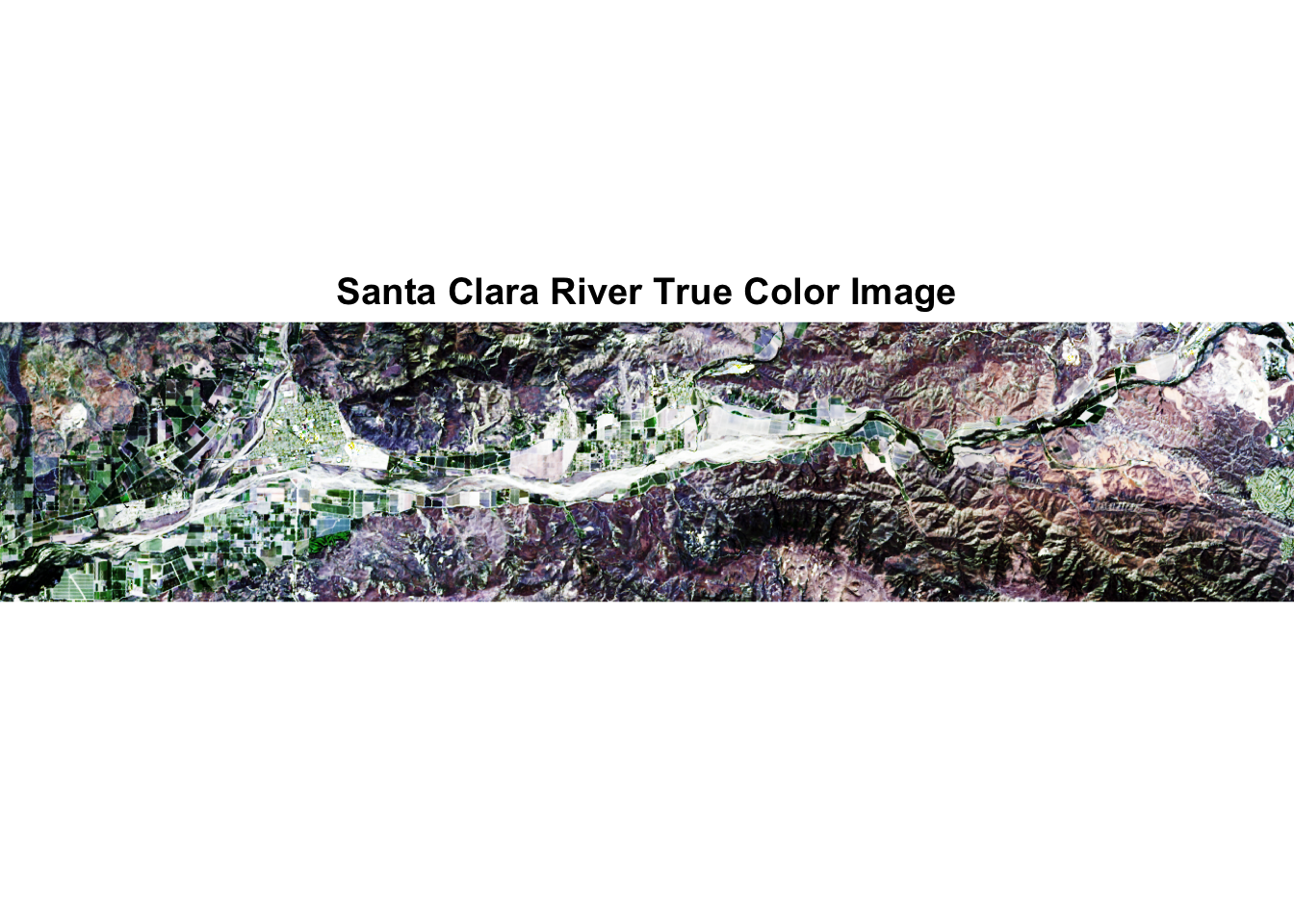

Study Site Location Along Santa Clara Watershed

The Santa Clara River flows from Santa Clarita to Ventura and remains relatively natural compared to other rivers in California. It is recognized for its ecological importance and natural resource potential, as the river provides water for agriculture and habitat for several endangered species. For these reasons, there have been significant efforts to conserve and restore the riparian habitat surrounding the river¹.

The following visualization depicts the Santa Clara River, as well as other rivers within the Santa Clara Watershed. The plant communities (study sites) were added as well for geographical context.

## ========== Data Preparation ==========
# filter VC river data to SC watershed
sc_watershed <- vc_rivers %>% 
  filter(WATERSHED == "SANTA CLARA RIVER WATERSHED") %>% #filter
  st_transform(crs = 'epsg:32611') %>% #reproject
  st_crop(study_sites)

# filter state data to counties new watershed
ventura <- states %>% st_crop(study_sites) #crop county to watershed

# create custom color palette
phenology_pal <- c("#EAAC8B", "#315C2B", "#315C2B", "#315C2B","#9EA93F")

## ========== Plot Data Together ==========
# create map combining watershed, study sites, and counties
ggplot() +
  geom_sf(data = ventura, fill = '#E7DED9') +
  geom_sf(data = sc_watershed, color = 'dodgerblue') +
  geom_sf(data = study_sites,
          mapping = aes(fill = study_site)) +
  scale_fill_manual(values = phenology_pal) +
  labs(title = "Study Sites Along Santa Clara Watershed",
       fill = "Plant Communities",
       x=NULL,
       y=NULL) +
  theme(panel.background = element_rect(fill='lightblue'),
        plot.margin=grid::unit(c(0,0,0,0), "mm"))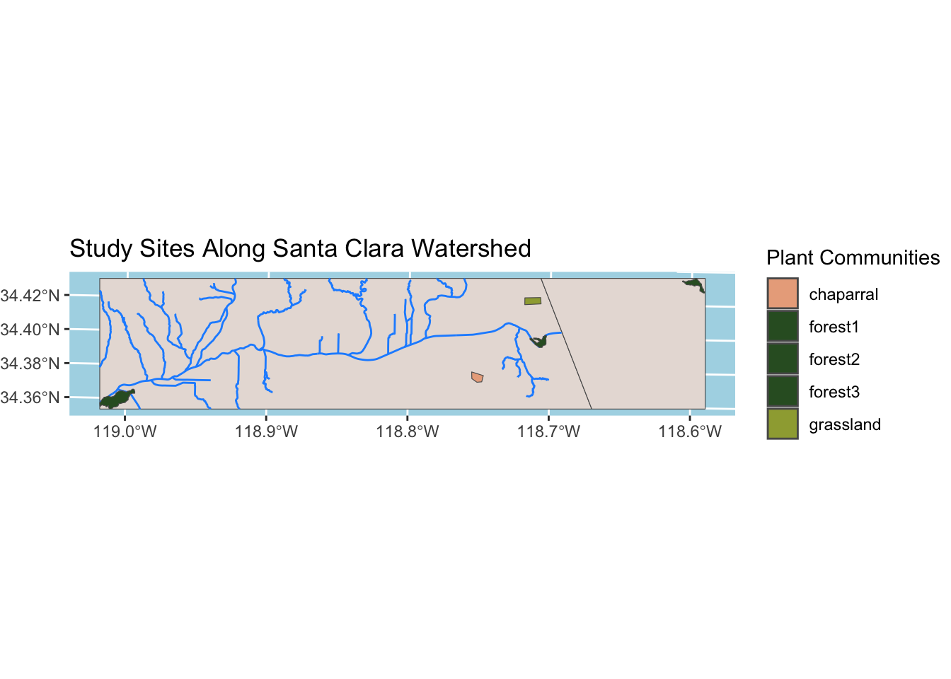

Study Sites and NDVI

This map demonstrates study sites within a single NDVI layer. For simplicity, I will call the first layer from the all_ndvi raster stack.

tm_shape(all_ndvi[[1]]) +
  tm_raster() +
  tm_shape(study_sites) +
  tm_polygons()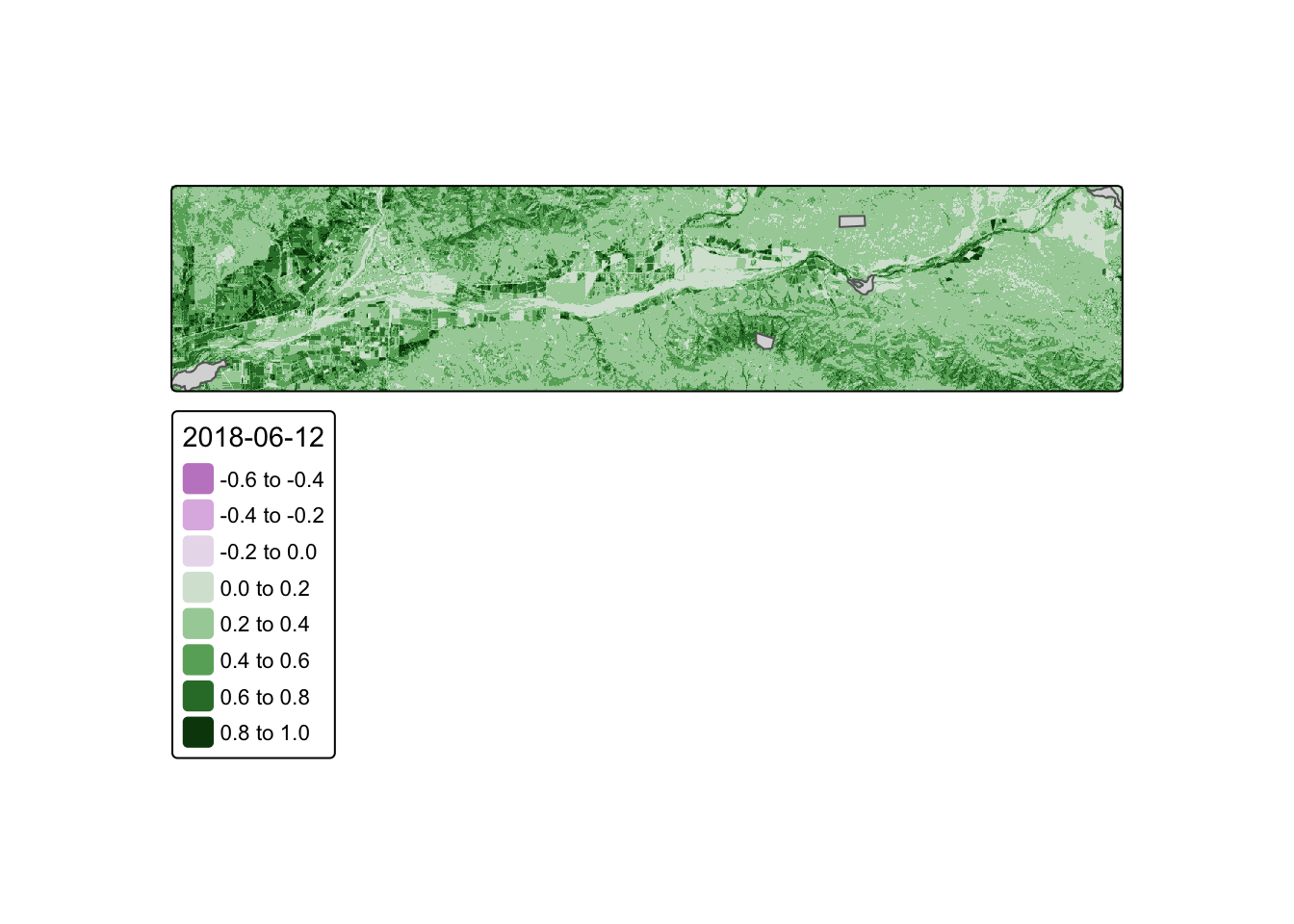

The normalized vegetation index (NDVI) can be used to estimate plant productivity. Areas with sparse foliage will return lower values, while areas with dense leaf cover will return values closer to 1. The NDVI scale ranges from -1 to 1, but vegetation is commonly a positive value. A negative NDVI is indicative of water, either as clouds, snow, or bodies of water on the Earth’s surface. For this reason, cloud cover can potentially affect NDVI values calculated from remotely sensed data.

NDVI Within Study Sites

Data Cleaning

Before the final plot can be produced, the average NDVI within each study site must be isolated. This was done using the extract() function from the terra package, followed by cbind to combine NDVI values with the original study site data.

## ========== Find NDVI within sites ==========
# use extract to pull NDVI values
sites_ndvi <- terra::extract(all_ndvi, study_sites, fun = 'mean')

# bind site data w/ site specific NDVI
sites_ndvi_raw <- cbind(study_sites, sites_ndvi)

## ========== Clean Data frame =========
sites_clean <- sites_ndvi_raw %>% 
  st_drop_geometry() %>%
  select(-ID) %>%
  pivot_longer(!study_site) %>%
  rename("NDVI" = value) %>%
  mutate("year" = str_sub(name, 2, 5),
         "month" = str_sub(name, 7, 8),
         "day" = str_sub(name, -2, -1)) %>%
  unite("date", 4:6, sep = "-") %>%
  mutate("date" = lubridate::as_date(date))

Plot NDVI Over Time

Plotting NDVI over time can ideally give us insight into the phonological trends mentioned in the introduction. Typically, NDVI values will be lower in the winter when trees lose their leaves, and higher in the spring. Plotting all study sites together makes it easy to note differences in NDVI among different plant communities.

ggplot(sites_clean,
       aes(x = date, y = NDVI,
           group = study_site, col = study_site)) +
  scale_color_manual(values = phenology_pal) +
  geom_line() +
  theme_minimal() +
  labs(x = "", y = "Normalized Difference Vegetation Index (NDVI)", col = "Plant Communities",
       title = "Seasonal cycles of vegetation productivity")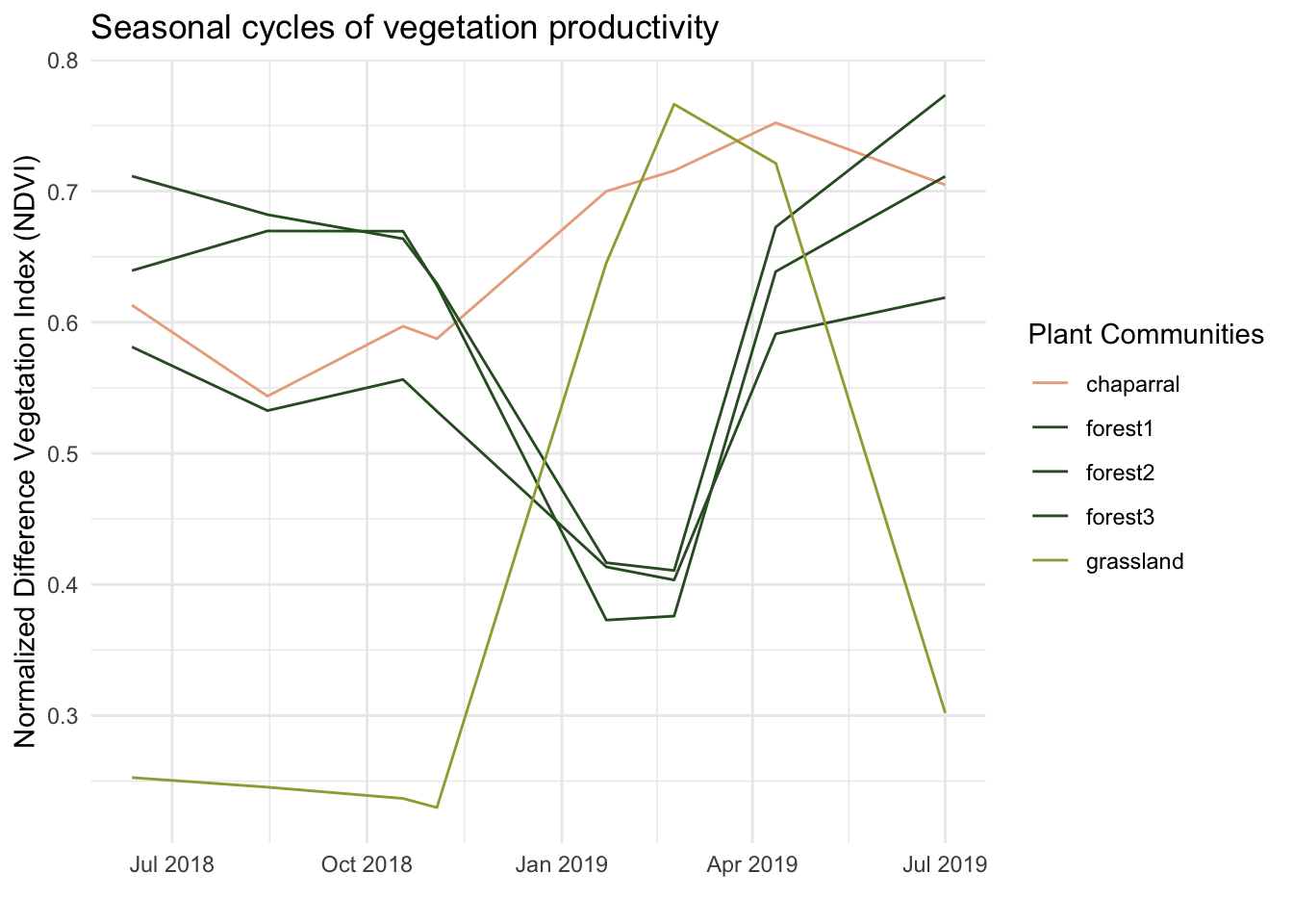 

Conclusion

Higher NDVI values often correlate with denser vegetation and times of rapid growth. Based on the plot produced, grasslands and chaparral sites appear to have faster growth in the springtime. Most notably, however, it appears that grasslands are ill equipped for winter as the NDVI from the end of 2018 is rather low. To expand this analysis, it would be useful to data beyond just one year. It is possible this year was not an accurate representation, and additional data would uncover this. With enough data, you could also minimize seasonal cycles to uncover trends that are only visible over several years.

Footnotes

1. “Santa Clara River.” The Nature Conservancy, www.nature.org/en-us/get-involved/how-to-help/places-we-protect/the-nature-conservancy-in-california-santa-clara-river-california-con/#:~:text=The%20Santa%20Clara%20River%20is%20a%20vital%20source%20of%20drinking,bustling%20Los%20Angeles%2DVentura%20region. Accessed 15 Dec. 2023.